How to use VLOOKUP in Excel

To use VLOOKUP, you have to first understand what it does and how it works. Then we will get to actually using it.

What does VLOOKUP do in Excel

The VLOOKUP function retrieves the value of a target cell located a specified number of columns to the right of a reference cell.

The format of the VLOOKUP function is as follows:

=VLOOKUP(lookup_value, table_array,col_index_num, [range_lookup])

VLOOKUP is the function. The stuff in the brackets are its inputs.

lookup_value: This defines the reference cell, or the search term for the row containing your target cell.

table_array: The area you are finding your reference and target cell in. Make sure both are within the area selection.

col_index_num: The number of columns to the right of the reference cell. The the cell located at this position is your target cell and what will be retrieved. The first column is 1.

[Range_lookup]: This is a 0 or 1 value to decide if you want to pick the first reference cell that matches the search term or if you want to find a perfect match. This is useful if your search term is a number with decimals.

How to use VLOOKUP with examples

Basic usage

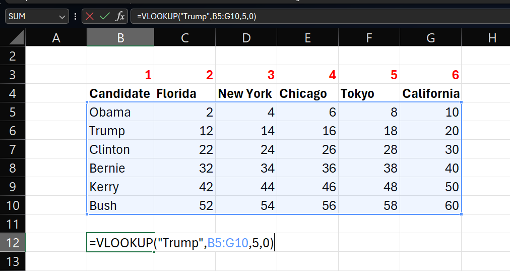
We have a table of votes each candidate got in different cities. We have also labelled the column numbers to help us find our target cell.

We want to retrieve the value of contained in Row: Trump, Column: Tokyo. Tokyo is in Column number 5.

The formula would therefore be =VLOOKUP(“Trump”,B5:G10,5,0). You don’t have to type B5:G10 manually. You can just drag across the cells you want. Just make sure that your Search term (Trump) and your target cell (Tokyo Votes) are within your selection. Notice how the column headings are not even part of the selection. We just need to know the column number.

Pressing enter gives the answer 18, which is exactly what is written in the 5th column of the row containing “Trump”.

Automate VLOOKUP for dragging

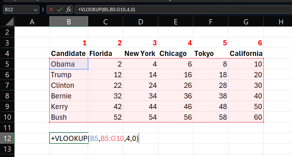
We can automate the VLOOKUP formula by setting our inputs to a cell reference rather than typing “Trump” like in the previous example.

Below we have selected the cell containing “Obama” but the formula reads =VLOOKUP(B5,B5:G10,4,0). This retrieves the value in the 4th column from where the row matches whatever value B5 contains.

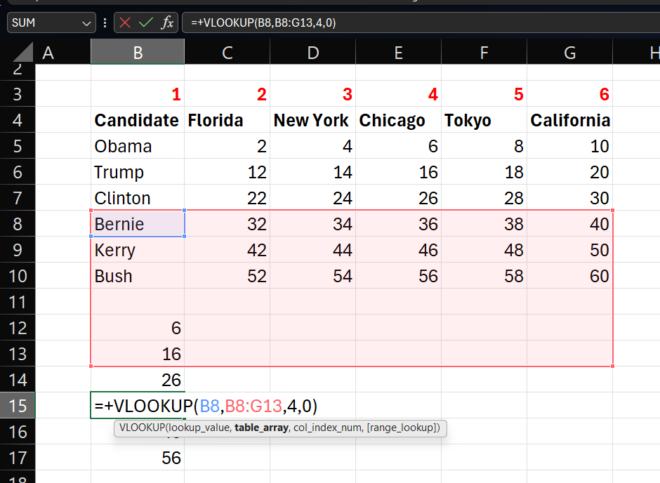
You could drag this formula down to get the results for other candidates/rows/searchterms. Note that dragging the formula down not only moves your reference cell, but also your selected area. This would cause #N/A errors when you drag far enough.

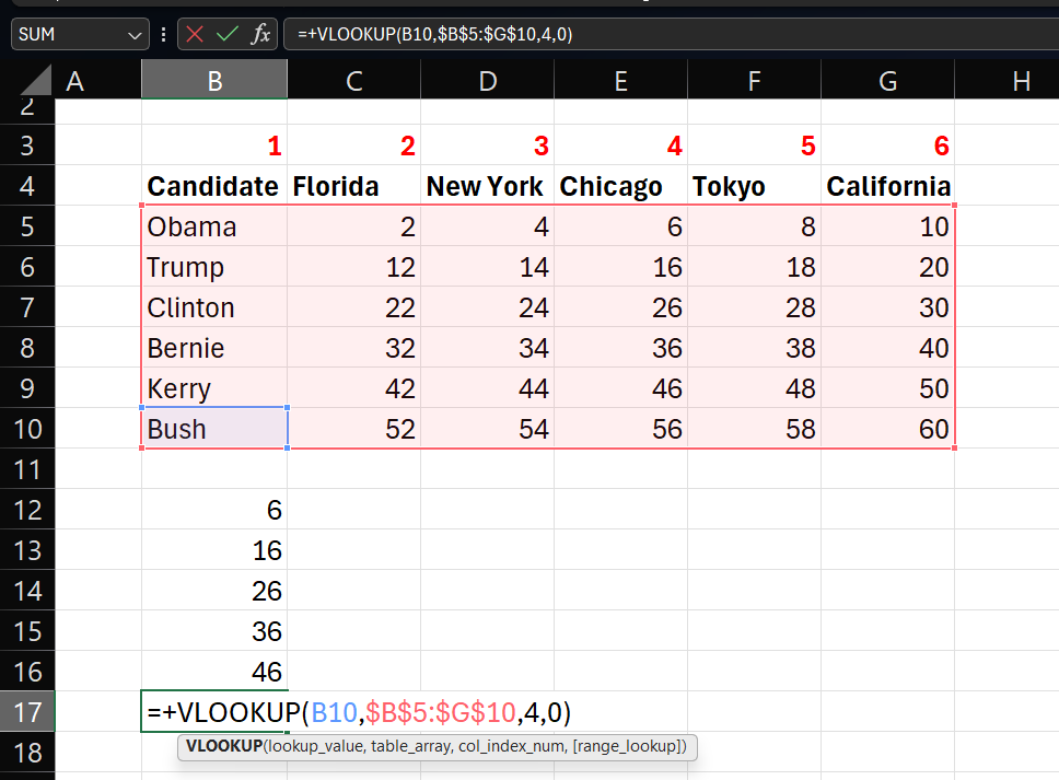
To prevent this, you can lock the array/area by adding a $ before its cell references. You could also move your cursor to the cell reference and press F4 a few times till a $ is placed before each character.

Now when you drag the formula, only the reference cell will move but your area will stay in place.